PivotTables and PivotCharts are fantastic Excel features that allow you to analyze data. Sometimes you need an easy way to manipulate only specific data and view it. This Trainer Tip will show you how to filter data in PivotTables and PivotCharts using Slicers.

Though you can filter data in a PivotTable using filters and by using the drop zones in the PowerPivot Field List pane, it may not be easy to understand what data you are looking for when multiple filters have been applied. Microsoft Excel provides Slicers to filter data with ease.

A Slicer is a filtering tool that provides you with options to include only the required elements in a PivotTable or PivotChart. Using Slicers, you can add and remove elements from a PivotTable or PivotChart so that data can be compared and evaluated from different perspectives. You can even create more than one slicer for a PivotTable or PivotChart. Slicers can be placed either on the same worksheet that contains the PivotTable or on a different worksheet.

Here’s how to do it:

Create a slicer in an existing PivotTable…

1. Click anywhere in the PivotTable for which you want to create a slicer.
2. On the PivotTable Analyze Contextual tab, click Insert Slicer.
3. In the Insert Slicers dialog box, select the check boxes of the PivotTable fields for which you want to create a slicer.
4. Click OK.

To integrate a slicer with your Pivot Chart,

1. Click anywhere in your pivot chart.
2. On the Analyze tab, in the Filter group, click Insert Slicer.
3. Select the checkboxes for the slicer(s) you want to create, and click OK.
4. If you’d like to delete the Slicer from the spreadsheet, just select it and then use the Delete key on your keyboard.

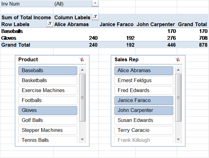
Here’s a picture of a PivotTable displaying data based on fields selected in slicers:

Learn all about Slicers in Full Circle Computing’s Excel PowerPivot/Excel Advanced Functions class!