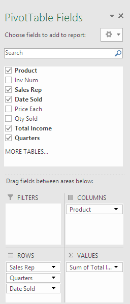
Automatic Time Grouping, a nice feature in Excel, helps use time-related fields in a PivotTable by auto-detecting and grouping them on your behalf.

The automatic grouping creates new Date/Time functionality and automatically populates the PivotTable in one action when you add a field to the ROWS or COLUMNS drop box in the PivotTable Task Pane. This allows users to quickly start analyzing their data across different levels of time with drill-down capabilities.

By clicking on a date field in the PivotTable Task Pane, the field moves by default to the ROWS drop box. You’ll then see the addition of date grouping intervals (e.g., Years, Quarters) appearing as fields in the ROWS drop box. If you then drag the date field to be a report FILTER (e.g., Date Sold), you won’t see the date displayed in the filter drop-down list but instead the Month of the date field.

Changing the Group Rows/Columns is always possible through the usual user interface. In the PivotTable, right-click the date field and select Group or Ungroup. The Group dialog box is where you can define other grouping intervals to be added or removed from the time group (Seconds, Minutes, Hours, Days, Months, Quarters, Years).

Don’t like automatic grouping?

Undo it just like you would any other applied change. The first undo (Ctrl+Z) removes the auto-added columns from the ROWS drop zone. The second undo removes the newly added ROWS so you are back at square one. Right-click Ungroup… is also supported and will act as if you have done the two undo operations, removing the group fields from the drop zones.

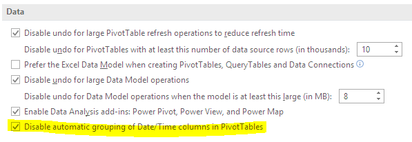
If you’d like to disable Automatic Time Group altogether in Excel 2016, go to the File menu, select Options, choose Advanced category, scroll down to the Data section and check “Disable automatic group of Date/Time columns in PivotTables.”

Come to Full Circle Computing to learn more about the power of Excel PivotTables and Data Management Techniques!!